
Hello Learners…
Welcome to my blog…
Table Of Contents
- Introduction
- OpenCV Python Full Tutorial For Data Science
- What is OpenCV?
- OpenCV Installation
- Reading And Displaying Images Using OpenCV And Python
- Image Resize Using OpenCV And Python
- Simple Thresholding On Images Using Python And OpenCV
- What is Thresholding?
- Types Of Thresholding
- Summary
- References
Introduction
In this post, we are going to learn OpenCV techniques that are used in image processing and used in real-world computer vision-based applications. There are many real-world applications in which images are involved and in processing that images we have to use OpenCV.OpenCV helps us in image processing. this is a huge library and very simple to use it. Thresholding is part of image processing.
Here, We see how we can apply Image Thresholding Using Python and OpenCV.
OpenCV Python Full Tutorial For Data Science
What Is OpenCV?
OpenCV is a library in the field of computer vision that will help us to achieve many many tasks like image processing or video processing here we understand some concepts of Opencv.
Opencv is a very vast library and we can use it with C, C++, Or Python. Documentation is very easy to understand and also code is very easy to understand
There are lots of functions like face detection that will help us to detect the face and then we can easily recognize it.
So OpenCV will help us in many many applications of computer vision.
Here are the applications of computer vision.
- Face Recognition
- Object Detection
- Object Classification
- Image Recognition
- Pattern Recognition
- Robotics
OpenCV Installation
First, we have to install OpenCV using the pip command.
pip install opencv-pythonwe can check our OpenCV version using the below code.
import cv2

cv2.__version__
Reading And Displaying Images Using OpenCV And Python
Reading Images and display in new windows
import cv2

image_path="./cat.jpg"

img=cv2.imread(image_path)


cv2.imshow(winname="Test Image",mat=img)
cv2.waitKey(0)
cv2.destroyAllWindows()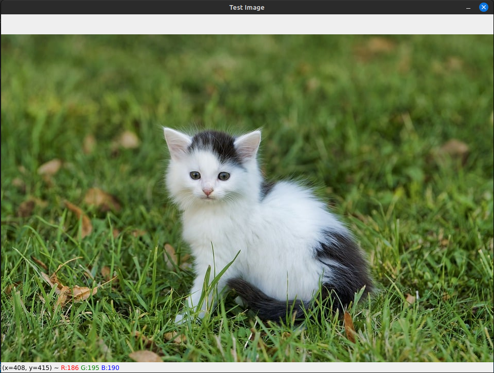
Display Images With Flags
Flags
- To read the image in RGB color flag=1 by default, cv2.IMREAD_COLOR
- To read the image in gray color flag=0, cv2.IMREAD_GRAYSCALE
- To read the image as it is flag=-1,cv2.IMREAD_UNCHANGED
import cv2

image_path="./cat.jpg"
img=cv2.imread(image_path,flags=0)


cv2.imshow(winname="Test Image",mat=img)
cv2.waitKey(0)
cv2.destroyAllWindows()
Image Resize Using OpenCV And Python
Image resizing is part of image processing. when we are working on images we must resize images in one size which will give us the best result.
Resize Image Using Pixels Values
import cv2

width=300
height=400
dimension=(width,height)

orig_img=cv2.imread(filename="cat.jpg",flags=1) #rgb
resize_img=cv2.resize(dsize=dimension,src=orig_img)


cv2.imshow(winname="Original Image",mat=orig_img)
cv2.imshow(winname="Resize Image",mat=resize_img)


cv2.waitKey(0)
cv2.destroyAllWindows()

Percentage Wise Resize
When we want to resize an image percentage wise like 50% smaller or 50% bigger than the original image or 2 times bigger or 2 times smaller.
here we define value of fx(width) and fy(height).here we set the value of fx=0.5 and fy=0.5 which means that we want to resize our image to 50% smaller than the height and width of the original one.
And here we have to set the value of dsize=(0,0).
import cv2


#fx means Width and fy means Height
img=cv2.imread(filename="cat.jpg",flags=1) #rgb

resize_img=cv2.resize(dsize=(0,0),src=img,fx=0.5,fy=0.5)


cv2.imshow(winname="Test Image",mat=img)
cv2.imshow(winname="Resize Image",mat=resize_img)


cv2.waitKey(0)
cv2.destroyAllWindows()
when we set the value of dsize=(200,200). It will consider that parameter for the resize.
import cv2


#fx means Width and fy means Height
img=cv2.imread(filename="cat.jpg",flags=1) #rgb

resize_img=cv2.resize(dsize=(200,200),src=img,fx=2,fy=2)


cv2.imshow(winname="Original Image",mat=img)
cv2.imshow(winname="Resize Image",mat=resize_img)


cv2.waitKey(0)
cv2.destroyAllWindows()
Save The Image Using OpenCV And Python
If we want to save any image then we can use imwrite() the function of OpenCV.
let’s take an example, we want to resize an image and save it as a different image then we can use imwrite() function.
It saves images at the given path.
import cv2

width=300
height=400
dimension=(width,height)

orig_img=cv2.imread(filename="cat.jpg",flags=1) #rgb
resize_img=cv2.resize(dsize=dimension,src=orig_img)
cv2.imwrite("resize_image.jpg",img=resize_img)
Convert The Color Of An Image Using OpenCV And Python
BGR TO GRAY
import cv2


cat_img=cv2.imread("cat.jpg",1)

cat_img_2=cv2.cvtColor(src=cat_img,code=cv2.COLOR_BGR2GRAY)
cv2.imwrite(filename="bgr2gray.jpg",img=cat_img_2)

BGR TO HSV
import cv2


cat_img=cv2.imread("cat.jpg",1)

cat_img_2=cv2.cvtColor(src=cat_img,code=cv2.COLOR_BGR2HSV)
cv2.imwrite(filename="bgr2hsv.jpg",img=cat_img_2)

Drawing On Images
As we know that an image is nothing but a bunch of pixels.
if our image shape is 100*150(width*height) then the total pixels are 15000 and every pixel has a unique value as per its color ranging between 0 to 255.
If it’s 3 Channel Image(RGB) then it looks like the below,
To Draw on images first we need to access that pixel’s values at the point we want to draw.
Here to show images we use matplotlib library which can be installed using pip.
pip install matplotlibAccessing Pixel Values
This is the image we used for image processing.
import matplotlib.pyplot as plt
import cv2

cat_img=cv2.imread("cat.jpg",1)
plt.imshow(cat_img)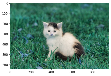
Here is a simple example of how we can access the pixel values of an image.
import cv2
import matplotlib.pyplot as plt

cat_img=cv2.imread("cat.jpg",1)
plt.imshow(cat_img[200:500,200:700])
Change The Values Of Pixels
Here we are going to change the values of some pixels of an image
import cv2
import matplotlib.pyplot as plt


cat_img=cv2.imread("cat.jpg",1)

#pixels values change
cat_img[200:500,200:700]=0

#0 is for black
plt.imshow(cat_img)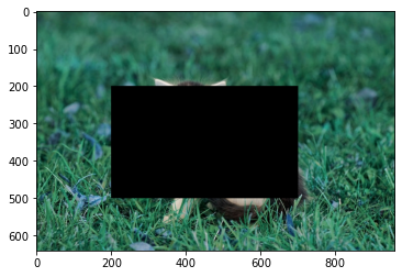
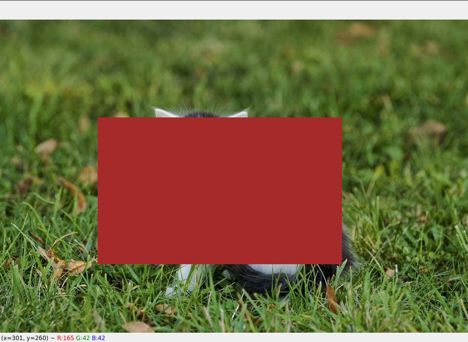
Opencv takes BGR if we change the pixels values
Brown Color For OpenCV =[42,42,165]
Matplotlib takes RGB color
Dark Blue color For matplotlib = [42,42,165]
import cv2
import matplotlib.pyplot as plt

cat_img=cv2.imread("cat.jpg",1)

#brown color
cat_img[200:500,200:700]=[42,42,165]

#Show Dark Blue Color
plt.imshow(cat_img) 
If we read the above image using OpenCV then we get as below.
Simple Thresholding On Images Using Python And OpenCV
What is Thresholding?
In a simple way threshold value means a specific point or value, and based on that specific pixel point or value we implement some operations on images.
Types Of Thresholding
There are mainly two types of Image Thresholding
- Simple Thresholding
- Adaptive Thresholding
To apply simple thresholding on images we required Python and OpenCV installed on our system.
There are mainly Five different thresholding techniques we can apply to our image for image processing.
- Binary Threshold
- Binary Inverse Threshold
- Truncate Threshold
- To Zero Threshold
- To Zero Inverse Threshold
Binary Threshold
here we set the threshold value as 100 and the threshold type is binary(0,1), so any pixel value which is greater than or equal to 100 will turn into 255 and all the other pixel values turn into 0.
In the Output image either the pixel values are completely 0 or completely 255.
import cv2


cat_img=cv2.imread("cat.jpg",1)

ret,thresh=cv2.threshold(src=cat_img,thresh=100,maxval=255,type=cv2.THRESH_BINARY)

cv2.imwrite(filename="binary_threshold.jpg",img=thresh)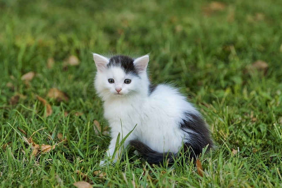

Here we can see the difference in the matrix values of both the images.
[[[ 49  97  79]
  [ 49  97  79]
  [ 49  97  79]
  ...
  [ 48 111  91]
  [ 47 110  90]
  [ 47 110  90]]

 [[ 47  95  77]
  [ 47  95  77]
  [ 47  95  77]
  ...
  [ 47 110  90]
  [ 47 110  90]
  [ 46 109  89]]

 [[ 45  93  75]
  [ 45  93  75]
  [ 45  93  75]
  ...
  [ 47 110  90]
  [ 46 109  89]
  [ 46 109  89]]

 ...

 [[ 69 140 113]
  [ 66 138 108]
  [ 54 128  98]
  ...
  [ 68 146 105]
  [ 67 143 101]
  [ 65 142  98]]

 [[ 54 125  98]
  [ 55 127  97]
  [ 52 126  96]
  ...
  [ 64 144 101]
  [ 64 143  99]
  [ 64 144  97]]

 [[ 40 111  84]
  [ 47 119  89]
  [ 51 125  95]
  ...
  [ 59 142  97]
  [ 62 143  98]
  [ 64 145  98]]]
[[[ 0 0 0]
[ 0 0 0]
[ 0 0 0]
...
[ 0 255 0]
[ 0 255 0]
[ 0 255 0]]
[[ 0 0 0]
[ 0 0 0]
[ 0 0 0]
...
[ 0 255 0]
[ 0 255 0]
[ 0 255 0]]
[[ 0 0 0]
[ 0 0 0]
[ 0 0 0]
...
[ 0 255 0]
[ 0 255 0]
[ 0 255 0]]
...
[[255 255 0]
[255 255 0]
[ 0 255 0]
...
[255 255 0]
[255 255 0]
[ 0 255 0]]
[[ 0 255 0]
[ 0 255 0]
[ 0 255 0]
...
[255 255 0]
[ 0 255 0]
[ 0 255 0]]
[[ 0 255 0]
[ 0 255 0]
[ 0 255 0]
...
[ 0 255 0]
[ 0 255 0]
[ 0 255 0]]]Binary Inverse Threshold
here we set the threshold value as 100 and the threshold type is the binary inverse(0,1), so any pixel value which is greater than or equal to 100 will turn into 0 and all the other pixel values turn into 255.
here we can see either the pixel values are completely 0 or completely 255.
import cv2


cat_img=cv2.imread("cat.jpg",1)

ret,thresh=cv2.threshold(src=cat_img_2,thresh=100,maxval=255,type=cv2.THRESH_BINARY_INV)

cv2.imwrite(filename="binary_inv_threshold.jpg",img=thresh)
Here we can see the difference in the matrix values of both the images.
[[[ 49  97  79]
  [ 49  97  79]
  [ 49  97  79]
  ...
  [ 48 111  91]
  [ 47 110  90]
  [ 47 110  90]]

 [[ 47  95  77]
  [ 47  95  77]
  [ 47  95  77]
  ...
  [ 47 110  90]
  [ 47 110  90]
  [ 46 109  89]]

 [[ 45  93  75]
  [ 45  93  75]
  [ 45  93  75]
  ...
  [ 47 110  90]
  [ 46 109  89]
  [ 46 109  89]]

 ...

 [[ 69 140 113]
  [ 66 138 108]
  [ 54 128  98]
  ...
  [ 68 146 105]
  [ 67 143 101]
  [ 65 142  98]]

 [[ 54 125  98]
  [ 55 127  97]
  [ 52 126  96]
  ...
  [ 64 144 101]
  [ 64 143  99]
  [ 64 144  97]]

 [[ 40 111  84]
  [ 47 119  89]
  [ 51 125  95]
  ...
  [ 59 142  97]
  [ 62 143  98]
  [ 64 145  98]]]
[[[255 255 255]
[255 255 255]
[255 255 255]
...
[255 0 255]
[255 0 255]
[255 0 255]]
[[255 255 255]
[255 255 255]
[255 255 255]
...
[255 0 255]
[255 0 255]
[255 0 255]]
[[255 255 255]
[255 255 255]
[255 255 255]
...
[255 0 255]
[255 0 255]
[255 0 255]]
...
[[ 0 0 255]
[ 0 0 255]
[255 0 255]
...
[ 0 0 255]
[ 0 0 255]
[255 0 255]]
[[255 0 255]
[255 0 255]
[255 0 255]
...
[ 0 0 255]
[255 0 255]
[255 0 255]]
[[255 0 255]
[255 0 255]
[255 0 255]
...
[255 0 255]
[255 0 255]
[255 0 255]]]Truncate Threshold
here we set the threshold value as 100 and the threshold type is truncated, so any pixel value which is greater than or equal to 100 will turn into 100, and all the other pixel values remain as it is.
import cv2


cat_img=cv2.imread("cat.jpg",1)
ret,thresh=cv2.threshold(src=cat_img_2,thresh=100,maxval=255,type=cv2.THRESH_TRUNC)

cv2.imwrite(filename="truncate_threshold.jpg",img=thresh)
Here we can see the difference in the matrix values of both the images.
[[[ 49  97  79]
  [ 49  97  79]
  [ 49  97  79]
  ...
  [ 48 111  91]
  [ 47 110  90]
  [ 47 110  90]]

 [[ 47  95  77]
  [ 47  95  77]
  [ 47  95  77]
  ...
  [ 47 110  90]
  [ 47 110  90]
  [ 46 109  89]]

 [[ 45  93  75]
  [ 45  93  75]
  [ 45  93  75]
  ...
  [ 47 110  90]
  [ 46 109  89]
  [ 46 109  89]]

 ...

 [[ 69 140 113]
  [ 66 138 108]
  [ 54 128  98]
  ...
  [ 68 146 105]
  [ 67 143 101]
  [ 65 142  98]]

 [[ 54 125  98]
  [ 55 127  97]
  [ 52 126  96]
  ...
  [ 64 144 101]
  [ 64 143  99]
  [ 64 144  97]]

 [[ 40 111  84]
  [ 47 119  89]
  [ 51 125  95]
  ...
  [ 59 142  97]
  [ 62 143  98]
  [ 64 145  98]]]
[[[ 79 97 49]
[ 79 97 49]
[ 79 97 49]
...
[ 91 100 48]
[ 90 100 47]
[ 90 100 47]]
[[ 77 95 47]
[ 77 95 47]
[ 77 95 47]
...
[ 90 100 47]
[ 90 100 47]
[ 89 100 46]]
[[ 75 93 45]
[ 75 93 45]
[ 75 93 45]
...
[ 90 100 47]
[ 89 100 46]
[ 89 100 46]]
...
[[100 100 69]
[100 100 66]
[ 98 100 54]
...
[100 100 68]
[100 100 67]
[ 98 100 65]]
[[ 98 100 54]
[ 97 100 55]
[ 96 100 52]
...
[100 100 64]
[ 99 100 64]
[ 97 100 64]]
[[ 84 100 40]
[ 89 100 47]
[ 95 100 51]
...
[ 97 100 59]
[ 98 100 62]
[ 98 100 64]]]To Zero Threshold
When we apply TOZERO_INV all the value less than the thresh values become 0. and others are remaining as it is.
import cv2


cat_img=cv2.imread("cat.jpg",1)

ret,thresh=cv2.threshold(src=cat_img_2,thresh=100,maxval=255,type=cv2.THRESH_TOZERO_INV)

cv2.imwrite(filename="tozero_inv_threshold.jpg",img=thresh) 
Here we can see the difference in the matrix values of both the images.
[[[ 49  97  79]
  [ 49  97  79]
  [ 49  97  79]
  ...
  [ 48 111  91]
  [ 47 110  90]
  [ 47 110  90]]

 [[ 47  95  77]
  [ 47  95  77]
  [ 47  95  77]
  ...
  [ 47 110  90]
  [ 47 110  90]
  [ 46 109  89]]

 [[ 45  93  75]
  [ 45  93  75]
  [ 45  93  75]
  ...
  [ 47 110  90]
  [ 46 109  89]
  [ 46 109  89]]

 ...

 [[ 69 140 113]
  [ 66 138 108]
  [ 54 128  98]
  ...
  [ 68 146 105]
  [ 67 143 101]
  [ 65 142  98]]

 [[ 54 125  98]
  [ 55 127  97]
  [ 52 126  96]
  ...
  [ 64 144 101]
  [ 64 143  99]
  [ 64 144  97]]

 [[ 40 111  84]
  [ 47 119  89]
  [ 51 125  95]
  ...
  [ 59 142  97]
  [ 62 143  98]
  [ 64 145  98]]]
[[[ 0 0 0]
[ 0 0 0]
[ 0 0 0]
...
[ 0 111 0]
[ 0 110 0]
[ 0 110 0]]
[[ 0 0 0]
[ 0 0 0]
[ 0 0 0]
...
[ 0 110 0]
[ 0 110 0]
[ 0 109 0]]
[[ 0 0 0]
[ 0 0 0]
[ 0 0 0]
...
[ 0 110 0]
[ 0 109 0]
[ 0 109 0]]
...
[[113 140 0]
[108 138 0]
[ 0 128 0]
...
[105 146 0]
[101 143 0]
[ 0 142 0]]
[[ 0 125 0]
[ 0 127 0]
[ 0 126 0]
...
[101 144 0]
[ 0 143 0]
[ 0 144 0]]
[[ 0 111 0]
[ 0 119 0]
[ 0 125 0]
...
[ 0 142 0]
[ 0 143 0]
[ 0 145 0]]]
To Zero Inverse Threshold
import cv2


cat_img=cv2.imread("cat.jpg",1)

ret,thresh=cv2.threshold(src=cat_img_2,thresh=100,maxval=255,type=cv2.THRESH_TOZERO_INV)

cv2.imwrite(filename="tozero_inv_threshold.jpg",img=thresh)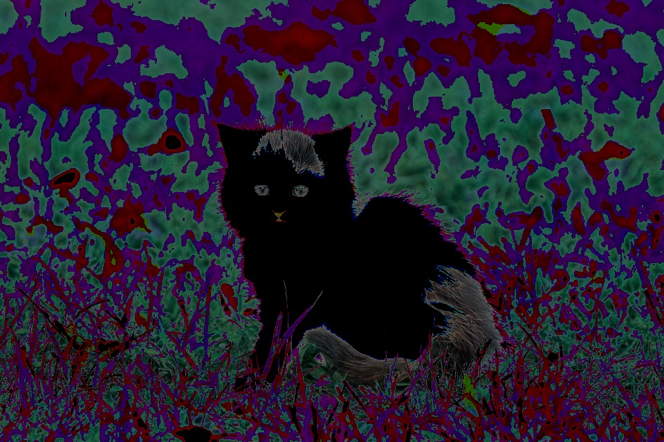
Here we can see the difference in the matrix values of both the images.
[[[ 49  97  79]
  [ 49  97  79]
  [ 49  97  79]
  ...
  [ 48 111  91]
  [ 47 110  90]
  [ 47 110  90]]

 [[ 47  95  77]
  [ 47  95  77]
  [ 47  95  77]
  ...
  [ 47 110  90]
  [ 47 110  90]
  [ 46 109  89]]

 [[ 45  93  75]
  [ 45  93  75]
  [ 45  93  75]
  ...
  [ 47 110  90]
  [ 46 109  89]
  [ 46 109  89]]

 ...

 [[ 69 140 113]
  [ 66 138 108]
  [ 54 128  98]
  ...
  [ 68 146 105]
  [ 67 143 101]
  [ 65 142  98]]

 [[ 54 125  98]
  [ 55 127  97]
  [ 52 126  96]
  ...
  [ 64 144 101]
  [ 64 143  99]
  [ 64 144  97]]

 [[ 40 111  84]
  [ 47 119  89]
  [ 51 125  95]
  ...
  [ 59 142  97]
  [ 62 143  98]
  [ 64 145  98]]]
[[[79 97 49]
[79 97 49]
[79 97 49]
...
[91 0 48]
[90 0 47]
[90 0 47]]
[[77 95 47]
[77 95 47]
[77 95 47]
...
[90 0 47]
[90 0 47]
[89 0 46]]
[[75 93 45]
[75 93 45]
[75 93 45]
...
[90 0 47]
[89 0 46]
[89 0 46]]
...
[[ 0 0 69]
[ 0 0 66]
[98 0 54]
...
[ 0 0 68]
[ 0 0 67]
[98 0 65]]
[[98 0 54]
[97 0 55]
[96 0 52]
...
[ 0 0 64]
[99 0 64]
[97 0 64]]
[[84 0 40]
[89 0 47]
[95 0 51]
...
[97 0 59]
[98 0 62]
[98 0 64]]]Summary
This is the simple thresholding on images using Python and OpenCV that we can use in image processing in our computer vision projects.
Download Full Source Code: https://github.com/galaxyofai/opencv_tutorial
Happy Learning And Keep Learning…
Thank You…
Also, you can refer to my other post related to computer vision.